图像旋转算法实现 Python
旋转原理
如下图,推导点\((x_0,y_0)\)旋转\(\theta\)到到点\((x,y)\),半径为R
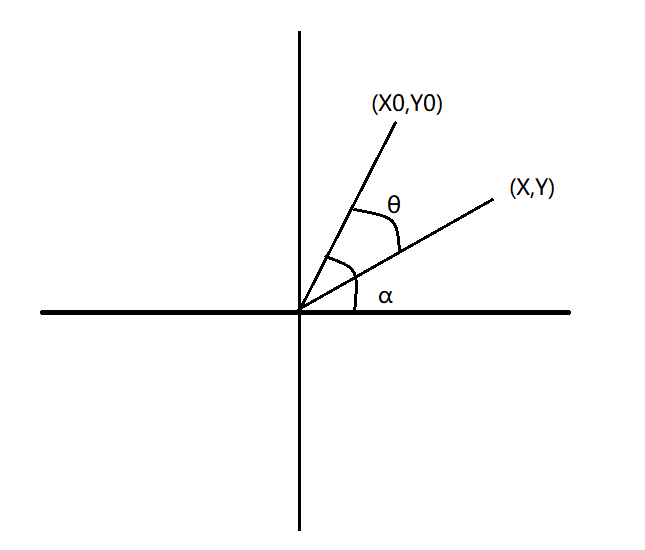
对于两点坐标可以这样表示:
\[ \begin{align} x_0 =& R*\cos\alpha \\ y_0 =& R*\sin\alpha \\ For:x\\ x =& R*\cos(\alpha-\theta) \\ =& R*(\cos\alpha\cos\theta+\sin\alpha\sin\theta) \\ =& x_0\cos\theta+y_0\sin\theta \\ For:y\\ y =& R*(\sin(\alpha-\theta)) \\ =& R*(\sin\alpha\cos\theta-\cos\alpha\sin\theta) \\ =& y_0\cos\theta-x_0\sin\theta \end{align} \]
使用矩阵表示有:
\[ \left[ \begin{matrix} x & y & 1 \end{matrix} \right]= \left[ \begin{matrix} x_0 & y_0 & 1 \end{matrix} \right] * \left[ \begin{matrix} \cos\theta & -\sin\theta & 0 \\ \sin\theta & \cos\theta & 0 \\ 0 & 0 & 1 \end{matrix} \right] \]
此为顺时针旋转\(\theta\) ,逆时针旋转\(\theta\)只需要将 \(\theta=-\theta\) 即可,易得:\((x,y)\rightarrow(x_0,y_0)\)
\[ \left[ \begin{matrix} x_0 & y_0 & 1 \end{matrix} \right]= \left[ \begin{matrix} x & y & 1 \end{matrix} \right] * \left[ \begin{matrix} \cos\theta & \sin\theta & 0 \\ -\sin\theta & \cos\theta & 0 \\ 0 & 0 & 1 \end{matrix} \right] \]
用于实际的旋转矩阵
上一部分的旋转矩阵是以数字坐标系推导的,而图像坐标系是以左上角为原点的图像坐标系,我们需要将图像坐标系转换为数字坐标系,方便的也需要从数字坐标系到图像坐标系的逆转换
假设原图片大小为\(W,H\),旋转后所包含图片的最小矩形大小为\(W^{'},H^{'}\)
设数字坐标系点为\((x,y)\)其相应的图像坐标系点为 \((x_0,y_0)\) 有如下表达式:
\[ \left[ \begin{matrix} x & y & 1 \end{matrix} \right]= \left[ \begin{matrix} x_0 & y_0 & 1 \end{matrix} \right] * \left[ \begin{matrix} 1 & 0 & 0 \\ 0 & -1 & 0 \\ -0.5W & 0.5H & 1 \end{matrix} \right] \]
\[ \left[ \begin{matrix} x_0 & y_0 & 1 \end{matrix} \right]= \left[ \begin{matrix} x & y & 1 \end{matrix} \right] * \left[ \begin{matrix} 1 & 0 & 0 \\ 0 & -1 & 0 \\ 0.5W^{'} & 0.5H^{'} & 1 \end{matrix} \right] \]
假设在图像坐标系中有点\((x_0,y_0)\)顺时针旋转\(\theta\) 到\((x,y)\)处转换后大小为\(W^{'},H^{'}\),转换公式有:
\[ \left[ \begin{matrix} x & y & 1 \end{matrix} \right]= \left[ \begin{matrix} x_0 & y_0 & 1 \end{matrix} \right] * \left[ \begin{matrix} 1 & 0 & 0 \\ 0 & -1 &0 \\ -0.5W & 0.5H & 0 \\ \end{matrix} \right] * \left[ \begin{matrix} \cos\theta & -\sin\theta & 0 \\ \sin\theta & \cos\theta & 0 \\ 0 & 0 & 1 \end{matrix} \right] * \left[ \begin{matrix} 1 & 0 & 0 \\ 0 & -1 & 0 \\ 0.5W^{'} & 0.5H^{'} & 1 \end{matrix} \right]\tag{1} \]
\[ \left[ \begin{matrix} x_0 & y_0 & 1 \end{matrix} \right]= \left[ \begin{matrix} x & y & 1 \end{matrix} \right] * \left[ \begin{matrix} 1 & 0 & 0 \\ 0 & -1 & 0 \\ -0.5W^{'} & 0.5H^{'} & 1 \end{matrix} \right] * \left[ \begin{matrix} \cos\theta & \sin\theta & 0 \\ -\sin\theta & \cos\theta & 0 \\ 0 & 0 & 1 \end{matrix} \right] * \left[ \begin{matrix} 1 & 0 & 0 \\ 0 & -1 &0 \\ 0.5W & 0.5H & 0 \\ \end{matrix} \right]\tag{2} \]
(1)式为前向映射(直接从原图映射到旋转后的图),(2)式为后向映射(用于旋转后映射到旋转前)
为什么需要后向映射而不是前向映射
之所以有后向映射是因为在前向映射中获取的旋转后坐标是浮点数,但是像素只能是整数,所以就产生了像素缺失
而从后向前映射像素信息都是存在的,但又存在映射到原图中的浮点坐标改如何选择颜色信息的问题
这就有内插值的问题,提供的解决办法有三个,最邻近内插、双线性内插、双三次内插,最邻近就是直接对浮点坐标取整,取最接近它的像素值,双线性内插就是取与它相邻的4个点,求线性渲染值
其本质就是:假设在数轴上有两个点A,B(A<B) AB中间有个点X,那么双线性内插就和知道X到点A的距离求X的值是一个道理,不过双线性需要对X和Y两个方向求值
双三次内插有点麻烦,这里。。我也不清楚,嘿嘿
可以参考https://blog.csdn.net/caomin1hao/article/details/81092134
Python 实践
所需外部库:
- numpy(矩阵计算)
- matplotlib (效果演示)
- skimage (只读取使用其内置图片 换cv2读自己图片也可以)
使用按像素遍历,比较耗时
后向映射中使用最邻近内插和双线性内插(双三次内插暂未处理)
1 | import numpy as np |
效果图展示

可以看出来双线性比最邻近好的多了
